Over the last two years, Pitt’s Robotics and Automation Society has supported a team for Mission 7 of the International Aerial Robotics Competition. For an introduction to the challenges of Mission 7, take a look at the IARC’s summary of the mission. We’ve made multiple posts about our progress along the way, including notes on our success at last year’s competition, all of which can be found on the RAS IARC project page. At the 2018 competition, we were awarded both “Best System Design” (for the design best suited to complete the mission) and “Best Technical Paper” (read our paper here) at the American Venue of the competition. Furthermore, we achieved the highest overall score at the American Venue.

Now that the project is complete, we wanted to write up a dump detailing the technical aspects of the project; that’s what this post is for. If you want to look at the interesting stuff we did and why we did it, read onward! (Or just skip to the part you’re interested in)

All of our code is open-source (most is free software, licensed under GPLv2) on GitHub in the Pitt-RAS organization. Many of the sections below have source files associated with them, listed as <repository name>/path/to/file. If you just want a list of all the repos for the project, they’re all here, under the iarc7 topic.

Behaviors Demonstrated

• Obstacle Avoidance
• Target Blocking
• Target Hitting
• Arena Boundary Bouncing

Hardware

• Frame
• Propulsion
• Sensors
• Compute

State Estimation

• Optical flow
• Extended Kalman Filter (EKF)
• Arena boundary detection

Controls

• Flight Controller
• Dynamic Thrust Model
• Motion Profile Controller

Target Robots

• Target Detection
• Target Filtering

Obstacles

• Obstacle Detection
• Obstacle Filtering
• Obstacle Avoidance

The things that didn’t work (if only we had another month)

• Grid-based Position Estimator
• Search-based Planner
• 6 Degree of Freedom UAV

Our team developed several high-level behaviors - although obstacle avoidance is the only one of these that was successfully demonstrated at competition, others were demonstrated in our test arenas. Here are a couple videos of successful runs:

Obstacle Avoidance Video

Here the drone pushes off of any obstacles that come too close to it, maintaining a safe distance. When no obstacles are nearby, it just hovers in place:

Target Blocking Video

Here the drone searches for a target, tracks it, blocks it, and returns to its starting position, fully autonomously:

Target Hitting Video

Here the drone tracks a target, and then instead of blocking it, the drone lands on top of the target to press the top switch:

Arena Boundary Bouncing Video

In this video, the drone flies autonomously in a constant direction, but when it detects that it has hit a boundary of the arena (the gray floor), it bounces off and moves in a new direction until it hits another boundary:

Our team put a lot of time into building a custom drone for this competition. Why did we do this? We have a couple of reasons which are intimately tied together. We wanted nearly full RGBD camera coverage around the bottom and sides of the drone, and all computation done onboard; the only commercially available system which was close to our design goals while fitting inside the competition size limit is the DJI M100 when used with the DJI Guidance camera system. We chose not to use this platform because it did not have quite enough thrust to carry the amount of compute we wanted available on the drone. So, we built a custom system.

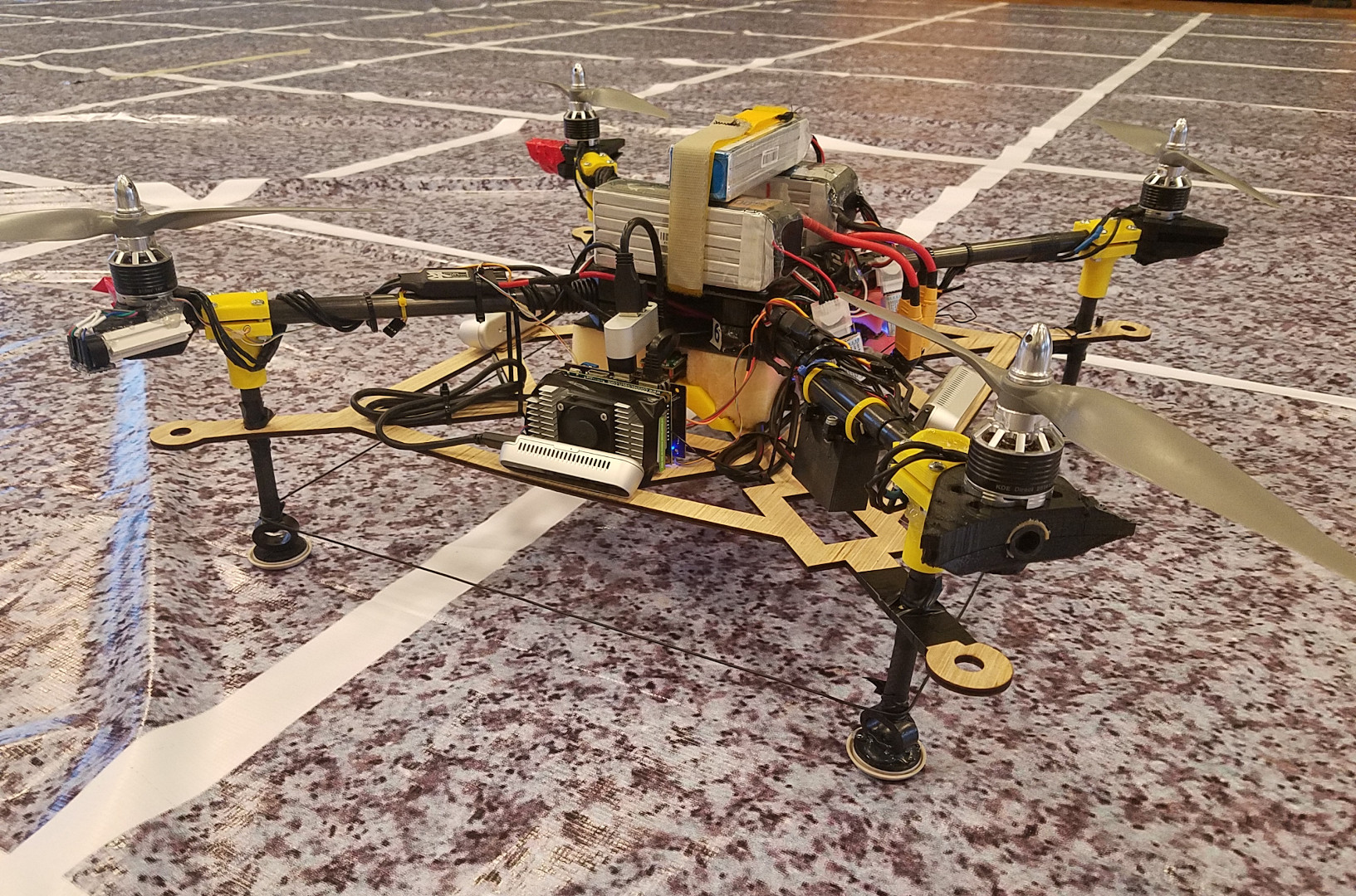
2018 Competition Drone

Frame

The frame is largely the same as our UAV’s in 2017, with a couple of major changes. First, the 2018 drone does not have prop guards. The primary reason for this was to save weight; the motors on the final drone were at their limit for power usage. Increasing the weight of the drone would have drastically decreased our flight time and control authority. Furthermore, the team was much more confident in the reliability of our software system this year, so we were comfortable flying without the extra protection of the prop guards.

The other major difference is the structure around the bottom of the drone. Because we switched from a scanning LIDAR to depth cameras this year, we no longer needed a plastic cage between the core of the drone and the target interaction plate to hold the LIDAR. Instead, a block of foam for shock absorbtion was mounted directly onto the core carbon fiber plate. We were also able to mount our sensors and compute on the bottom plate instead of on the core, providing a better weight distribution.

Several other changes were made for weight saving purposes; the bottom plate was made from laser cut plywood instead of cardboard, and the side bumpers for the targets were a single wire this year instead of wood.

Propulsion

The propulsion system this year is exactly the same as last year’s. We use four KDE Direct 515Kv motors with 12x6 APC propellors. The system is powered by two Tattu 6S1P 35C LiPo batteries in parallel.

Sensors

The drone is covered in a large montage of sensors. Some are only used for localization, such as the accelerometer and gyroscope inside the flight controller, as well as two LIDAR altimeters. We also included two time-of-flight LIDARs (a LidarLite v2 and a VL53L0X) to be used as altimeters because the LidarLite works well at altitudes above ~1m and the VL53L0X works well below this altitude, so we switch between them with a small transition region. Other than that, we have 6 cameras - a narrow-angle bottom camera (Intel Realsense R200), a wide-angle bottom camera (Leopard Imaging M021), and four depth cameras on the sides. These cameras perform various other functions, including localization, target detection, and obstacle detection.

Compute

We do all of our compution onboard. The primary computer is an NVIDIA Jetson TX2, which does all of the low-latency processing required for state estimation, target tracking, and control. The secondary computer is an Intel NUC 6i7KYK, which does all processing for the side cameras, which includes target detection, obstacle detection, and obstacle filtering. The two computers communicate over the network.

Optical Flow

Code: iarc7_vision/src/OpticalFlowEstimator.cpp

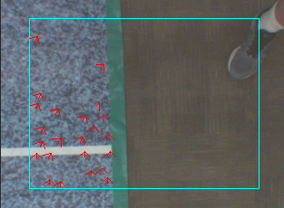
Picture of flow vectors and flow statistics - In the left image, red arrows are features detected in valid regions, meaning inside of the blue rectangle and outside of any green circles surrounding target robots. The right image is a visualization of flow vector statistics. Green points represent observed differences in feature locations between images, red ellipse represents distribution shape after outlier rejection, the yellow circle represents the variance of the remaining vectors, and the white circle represents maximum allowed variance of the filtered set

We chose to do velocity estimation using optical flow on our bottom camera instead of using an optical flow module such as the PX4Flow. This was primarily so that we could throw out flow from the moving targets, which would give us incorrect velocity estimates if we did not reject the target’s region from the frame. We use the Sparse PyrLK flow estimator in OpenCV, which provides flow vectors for a specified set of features between a pair of images. These flow vectors are then filtered for outlier rejection. Furthermore, if a frame does not have a tight enough distribution of flow estimates after outlier rejection, the entire frame is rejected.

Extended Kalman Filter (EKF)

We use the robot_localization state estimator, which uses an EKF to estimate 6DOF pose, 6DOF velocity, and translational acceleration. We modified the filter to only estimate the translational components, because we use the orientation estimates straight out of the flight controller orientation estimator.

Arena Boundary Detection

Code: iarc7_vision/src/iarc7_vision/floor_detector.py

An input to the arena boundary detector

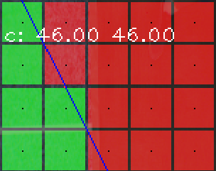
Green squares above were classified as arena floor, red squares were classified as other. The blue line is the calculated boundary.

The Arena Boundary detector is a texture classifier intended to distinguish the floor in the interior of the arena from other floor textures (such as that outside of the arena). We do this by splitting the image from the bottom camera into patches, and then classifying each patch separately as either “Arena floor” or “Other.” The classification is performed by first running an MR filter bank over the patch (with 3 added features for the average R, G, and B values of the patch), then using an SVM with an RBF kernel to classify the resulting feature vector. Then, we must extract a boundary line from the classified patches - we use some heuristics to throw out detections which are likely to be noise, then train a linear SVM on the resulting red/green points to find the boundary line in the image which best separates them.

Flight Controller

Code: iarc7_fc_comms, cleanflight branch:ras-cleanflight

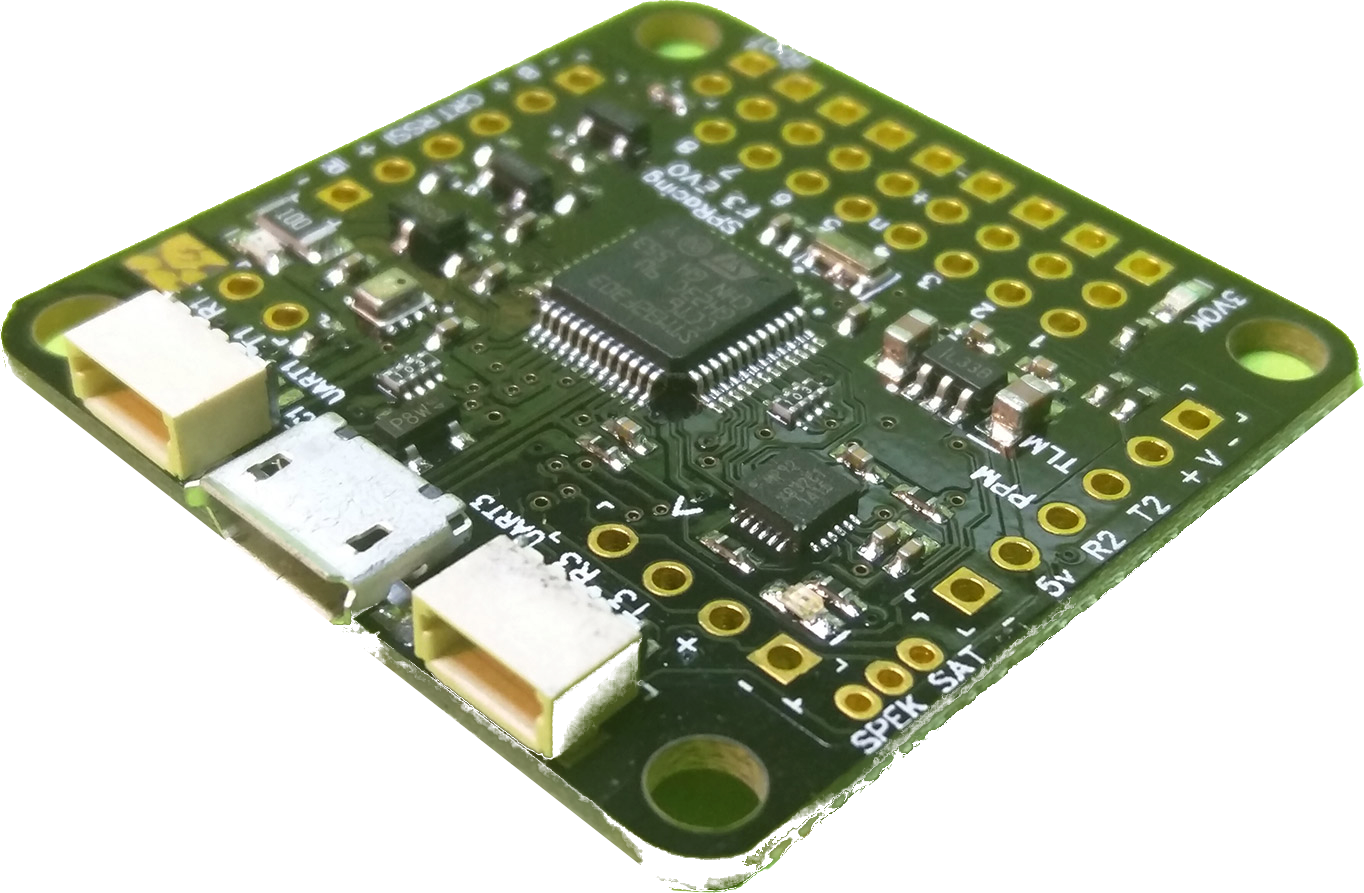
Seriously Pro F3 Evo flight controller

At the heart of the controls is the flight controller. We chose to use a Seriously Pro F3 Evo flight controller running Cleanflight. This flight controller is typically used for racing drones. It was chosen in 2016 when the project began. In the end, we believe this was a good choice.

The most popular alternative was a Pixhawk running either Ardupilot or PX4. Later on, we found that neither of those platforms were particularly suited to indoor flight. For instance, at the time, it was impossible to turn the magnetometer off in the EKF2 state estimator in PX4, perturbing indoor estimations. Additionally, the interfaces offered to the companion computer did not allow commanding a position and a velocity simultaneously. Finally, the takeoff proecedure in these systems was observed to be more suited to outdoor flight than indoor flight. We wanted to achieve precise control when taking off and landing, as these operations would need to be done repeatedly during Mission 7.

The Cleanflight firmware was modified in several important ways:

• Dual Receiver
  • Allowed receiving RX commands from a radio and from the autopilot via the MSP protocol simultaneously. This allowed a safety pilot to take over and fly the drone normally in the case of emergency.
• Seperate accelerometer low pass filter for state estimation
  • The low pass filter on accelerometer measurements used for orientation estimation within Cleanflight was not suitable for state estimation.
• Made the angle controller a full PID controller
  • The angular position controller was a proportional controller on top of a PID angular rate controller. We made the angular positional controller a PID controller on angular position cascaded with a PID controller on angular rate.

The flight controller sets an average throttle as commanded by the Jetson’s software via a serial interface. It then modulates the thrust to individual rotors to achieve a commanded orientation. Thus, the flight controller can stabilize orientation, but it cannot control position. This is handled by the dynamic thrust model and motion profile controller.

Dynamic Thrust Model

Code: iarc7_motion/scripts/thrust_model_v2, iarc7_motion/include/iarc7_motion/ThrustModel.hpp

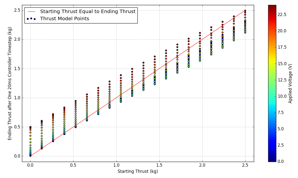
A thrust model visualized - Each point shows the thrust at the next timestep if the given voltage is applied at the current thrust. The red line shows when the current thrust is equal to the thrust at the next timestep. Colored dots indicate achievable thrusts and the voltage required given a starting thrust. Bilinear interpolation was used in the controller to fill in the gaps.

The throttle applied to a rotor does not linearly correspond to a thrust. In the 2016-2017 academic year, work was done to linearize the rotors using a steady-state thrust model that mapped a steady-state operating condition to a thrust. However, it was observed in the 2017-2018 year that significant performance gains could be achieved with a model that was aware of the current operating point of a rotor. Such a model could apply a voltage higher or lower than the steady state voltage in order to achieve a desired thrust more quickly.

Thus, a custom dynamic rotor model was derived and used. The model’s parameters are found using a form of system identification requiring a dynomometer stand capable of logging a rotors thrust and applied voltage over time. The response of the rotor to over 100 step impulses, linearly spaced over the entire throttle range, were used to find a mathmatical model that approximates the next achievable thrust based on the current thrust and an applied voltage. This process is demonstrated below:

In a manner similar to explicit model predictive control, the result of the model is precomputed for a wide range of starting voltages and starting thrusts. On the drone, the resulting approximation is searched in real time to find the optimal voltage to achieve a desired thrust in the next time step.

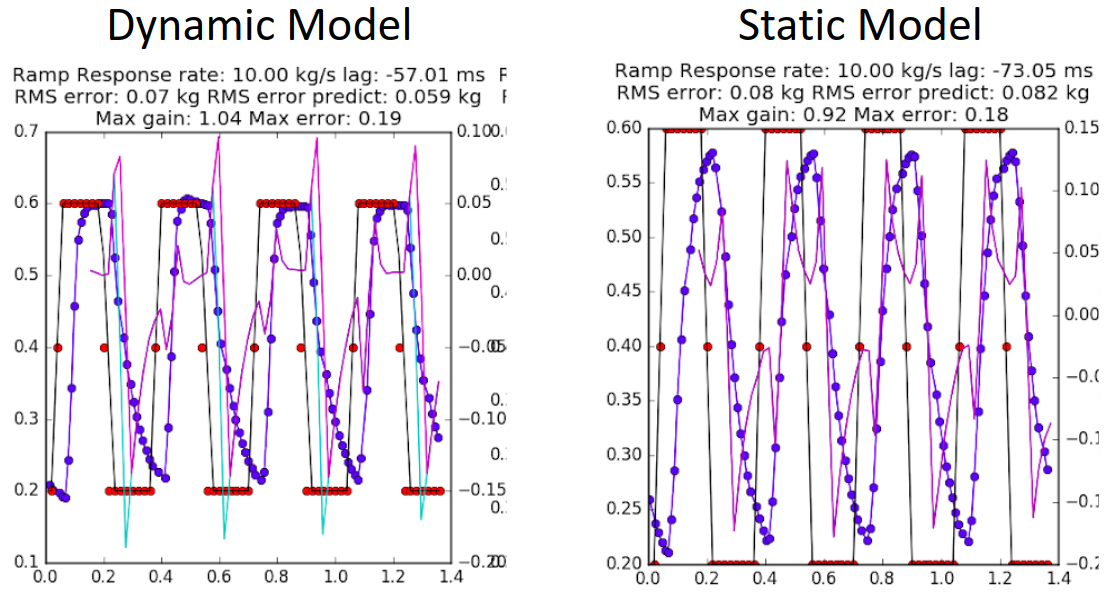
Example of the dynamic versus the static model performance for the same thrust profile
The commanded thrust profile (red) is trapezoidal with 10kg/s slew rates
The horizontal axis is time in seconds
The left vertical axis is thrust in kg/s

The dynamic thrust model provided several important benefits. It decreased rotor lag by as much as 80ms to 40ms. Thrust lag was fairly constant for all thrust slew rates (the steady state model saw considerable variation). Finally, it increased the maximum thrust slew rate by as much as four times. From a linear controls perspective, this greatly increased stability by increasing the gain and phase margins. Overall, it also improved the stability of the drone while holding height. It generally made the drone more responsive because feedforward of acceleration setpoints was possible.

Motion Profile Controller

Code: iarc7_motion/src/QuadVelocityController.cpp

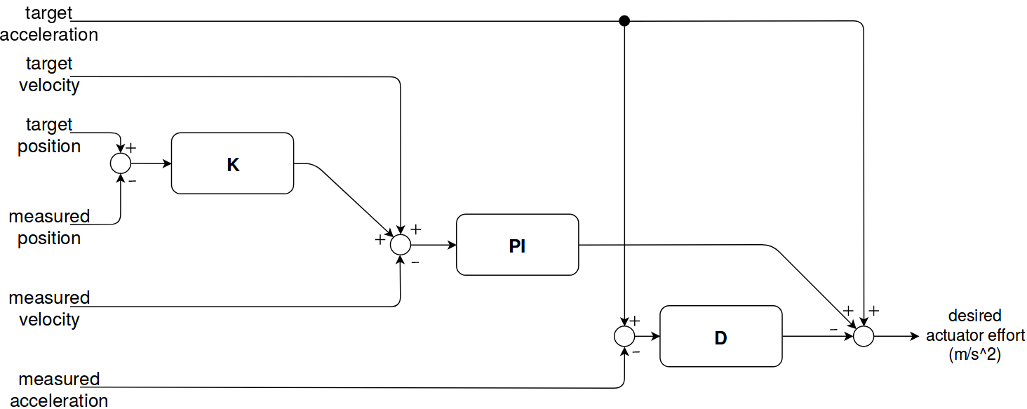
Controller diagram for a single axis of the motion profile controller

While, the Dynamic Thrust Model allowed the average rotor thrust to be accurately controlled, it did not correct for errors in position and velocity. For this, a linear controller was used. The above diagram shows the controller as used for a single axis. One of these controllers was independently run for the X, Y, and Z axis. This controller design was found through trial and error and is loosely based on the PX4 controller used at the time of writing. The main differences are that the PX4 controller does not allow for feedforward or multiple inputs as our controller did.

We called the controller a Motion Profile Controller because it accepted accepted a future stamped list of positions, velocities, and accelerations. It would the attempt to achieve the motion profile, while correcting for errors in position, velocity, and acceleration simultaneously.

The greatest benefit of this controller was the ability to use acceleration setpoints. This made the drone much more responsive than if the controller only accepted velocity setpoints. PX4 and Ardupilot did not support this feature at the time.

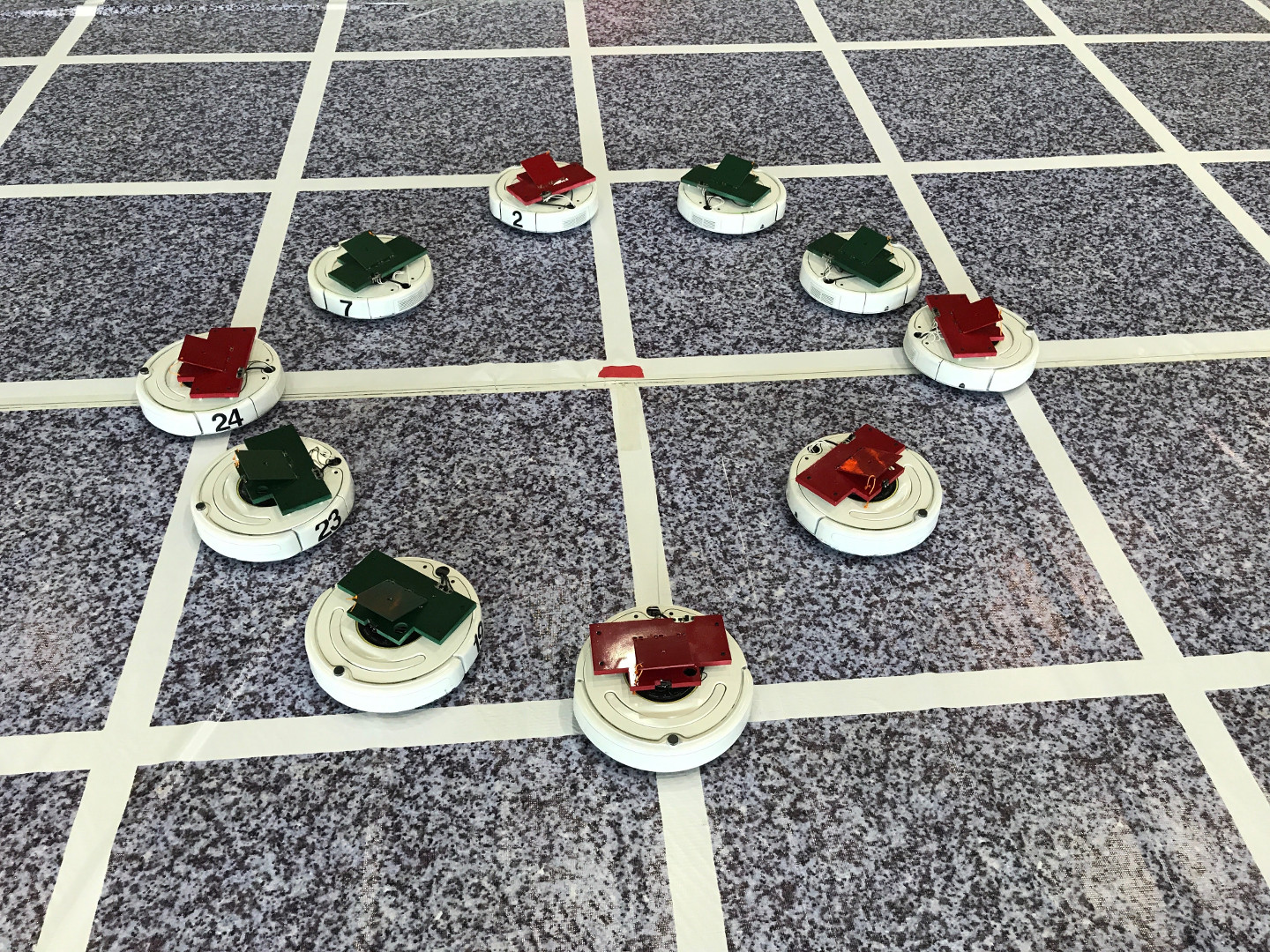
The IARC Target Robots

Target Detection

Code: iarc7_vision/src/RoombaEstimator.cpp, iarc7_vision_cnn/src/DarkflowRos.py

We have two vision-based detectors for finding the target robots - one which runs on the bottom camera, and one which runs on the side cameras.

Bottom Camera Detector

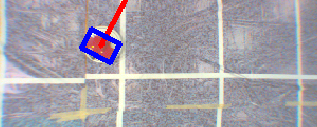
The detector on the bottom camera is based on classical computer vision techniques designed to find the colored top plates of the robots. It first converts the image to the HSV color space, then normalizes the saturation. The image is then thresholded in the HSV space to produce a binary image of pixels which are believed to belong to a top plate. Morphology operations are performed to get rid of extra noise pixels, and the boundaries of the resulting blobs are then found. We then find the covariance matrix and diagonalize it - because the top plates are rectangular, the eigenvector with the larger eigenvalue points along the long direction of the top plate. This gives us an oriented bounding box for the plate, but does not deal with rotations by 180 degrees.

To fix this, we then test the four corners of the plate where we expect the cutouts to be (as seen in the image above). Based on which corners are white, we are able to determine the direction of the front of the roomba exactly.

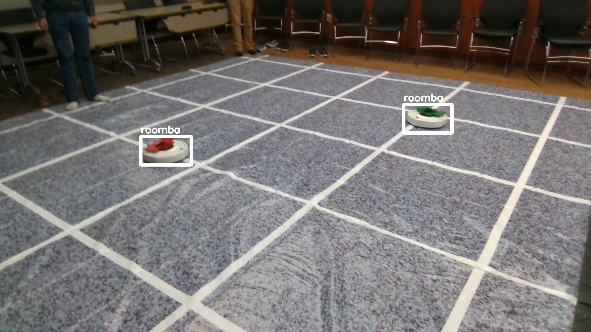
TinyYOLO Roomba Detector

The detector for the side cameras is a CNN based on the TinyYOLO architecture. We used the DarkFlow implementation of TinyYOLO in Tensorflow to train the model on approximately 3600 labeled examples.

Target Filtering

Code: iarc7_sensors/src/iarc7_sensors/roomba_filter.py

The target filter is a collection of multiple custom filters, one for each target that is currently being tracked. When a new measurement comes into the filter, it is first compared against all the targets the system is currently aware of. If it is close enough (defined by both physical distance and a p-test on the probability that the new measurement could have come from the current filter distribution), then the measurement is added into that single-target filter. Otherwise, a new target filter is added to the system. A variety of metrics are tracked to determine whether each single-target filter should be thrown out, including time since last measurement, statistical uncertainty in the target’s position, and a combination of how many times the target has been seen versus how many frames it was not detected in a frame where it should have been visible based on camera position.

Each single-target filter is a collection of two Kalman filters; one is a simple filter on the 2d position and velocity of the target, which is used when we don’t know the target’s orientation. Once the target’s orientation is known (either because the velocity is well-known or because the detector is confident about the target orientation as described above), the model switches to an EKF with a state space of position, heading, and yaw rate. The speed is fixed at the known speed of the target robots when they are moving.

Finally, the single-target filter has a mechanism for dealing with a target that is stopped and turning around by 180 degrees (which the targets do every 20 seconds). The filter keeps a history of measured positions, and attempts to fit a model of linear motion up to some stopping time for a set of possible stopping times. If, for any possible stopping time, the observed history is statistically better explained by the target stopping than continuing forward, the target speed is changed to 0 in the filter at that time and the yaw rate is set to the known constant yaw rate of the target robots.

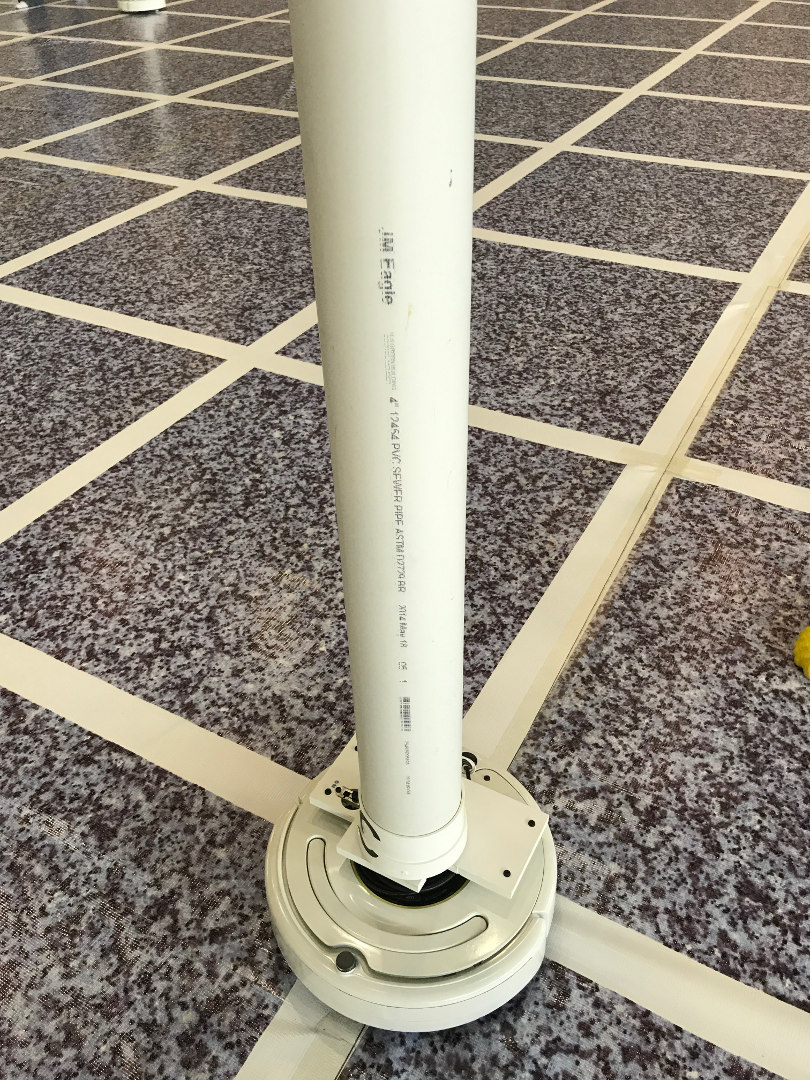
An IARC Obstacle Robot

IARC Mission 7 requires the drone to avoid several obstacle robots in the arena, as seen above. These obstacles primarily move in circles around the arena, although their movement is not very precise.

Obstacle Detection

Code: iarc7_sensors/src/iarc7_sensors/obstacle_detector_r200.py

Our obstacle detection is based on four Intel Realsense depth cameras, one pointing horizontally on each side of the UAV. Using depth cameras instead of a scanning LIDAR gives us a better vertical field of view - we can see obstacles below us that would not be seen by a planar LIDAR. Furthermore, we achieved better position estimates because the resolution on the depth cameras is superior to the scanning LIDARs in our price range; such as the RP-LIDAR A2 or the Scanse Sweep.

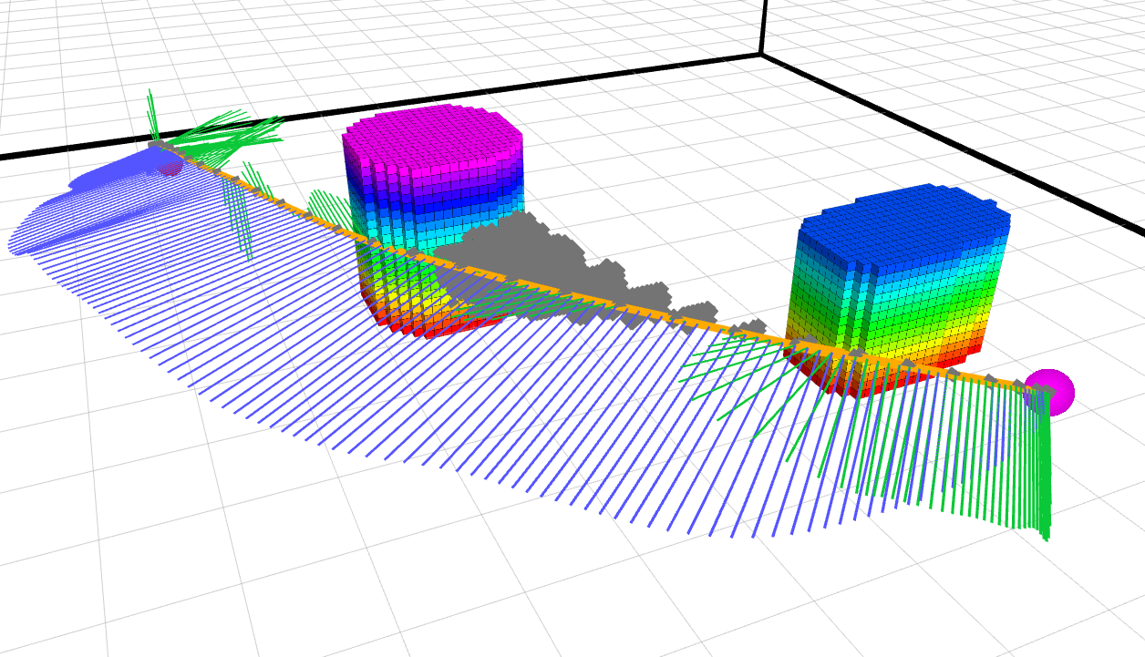
The detection algorithm first filters out points which do not belong to obstacles based on a variety of thresholds - these include throwing out the floor, throwing out points that are too far from the camera (because the noise in the depth map gets extremely large at long range), and throwing out points that are too close (because they are noise or they belong to the drone itself). The points left should all belong to the PVC pipe obstacles that we expect in the arena, pictured below:

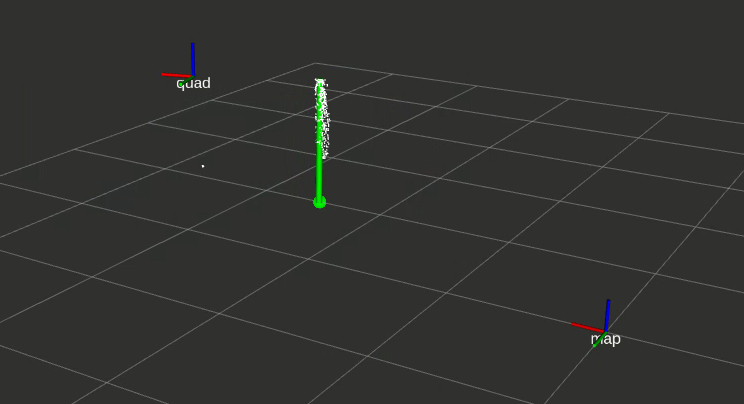
Obstacle Point Cloud - The green sphere at the bottom indicates the position estimate from the detector, and the green cylinder indicates the filtered obstacle position

To group these points into individual obstacles, we run the DBSCAN clustering algorithm. We then calculate the bounding box of each of the resulting clusters and report them as obstacle detections.

Obstacle Filtering

Code: iarc7_sensors/src/iarc7_sensors/obstacle_filter.py

The raw detections have several issues: they are noisy, they occasionally have false positives and false negatives, and there are blind spots around the drone. To fix these problems, we run a filter on top of these raw detections. The main filter is actually a collection of single-obstacle filters, just like the target tracking filter. It uses the same mechanisms for sorting obstacles into single-obstacle filters. The single-obstacle filters are then the same as the single-target filters, except that they never leave the naive position-velocity Kalman Filter. Even though we do have a more detailed motion model for the obstacles which would allow for a better filter, the position-velocity filter is good enough for our purposes, and it allows us to track obstacles other than the PVC roombas used in the IARC competition.

Obstacle Avoidance

Code: iarc7_motion/src/iarc7_motion/iarc_tasks/task_utilities/obstacle_avoid_helper.py

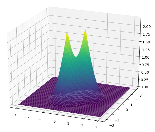
Obstacle Avoidance Potential Field

Obstacle avoidance is performed using a modified potential field like the one shown above, where the force generated by the field modifies the requested velocity from the current task. The primary difference from a typical potential field is that the distance between the drone and the obstacle is predicted forward in time based on the drone’s current velocity. Because the drone’s acceleration is severely limited relative to its maximum allowed velocity, this causes the drone to react sooner if it will take longer to decelerate and avoid the obstacle.

Grid-based Position Estimator

Code: iarc7_vision/src/GridLineEstimator.cpp

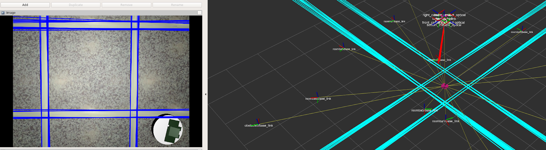
Grid Detector

The primary state estimation technique that we didn’t enable at the competition was a global position estimator based on the grid on the competition floor, which would have killed the drift in both our yaw estimates and position estimates. The grid detector we had implemented worked, but had problems with jumpy position estimates that made it unusable in some situations. The current implementation in the iarc7_vision repository uses an edge detector and a Hough transform to find the two edges of each white line in the arena, and then does a fitting procedure to minimize the squared difference in angle between the observed lines and the grid, followed by another fit to minimize the squared difference in position. The 1m translation and 90 degree rotation ambiguities this leaves are then resolved based on the current estimated pose of the drone. As you can see in the image, OpenCV’s Hough transform does not perform non-max suppression, so multiple detections are present for each line. Work was in progress here to both perform the non-max suppression and to detect the core of the line instead of the two edges, but that work was not finished in time for competiion.

Search-based planner

Code: iarc7_planner

Search-based Planner - Planned trajectory, including velocity in blue and acceleration in green, with expanded states in gray

We wanted to use a search-based planner to generate plans that satisfied our dynamic constraints while also avoiding obstacles. Our planner was based on the one described in Search-based Motion Planning for Quadrotors using Linear Quadratic Minimum Time Control, using a fork of the code that they provided here. In summary, the planner searches through a graph with edges defined as short trajectories which are optimal with respect to a combination of time and control effort. Obstacles are represented as a 3D occupancy grid; the drone is modeled as a sphere, so the occupied regions are simply inflated by the drone radius. The search used is a Weighted A*. The planner was able to consistently generate smooth plans well within the time constraint of 100ms, but suffered from some stability and integration issues which were not able to be resolved in time for competition.

6 Degree of Freedom UAV

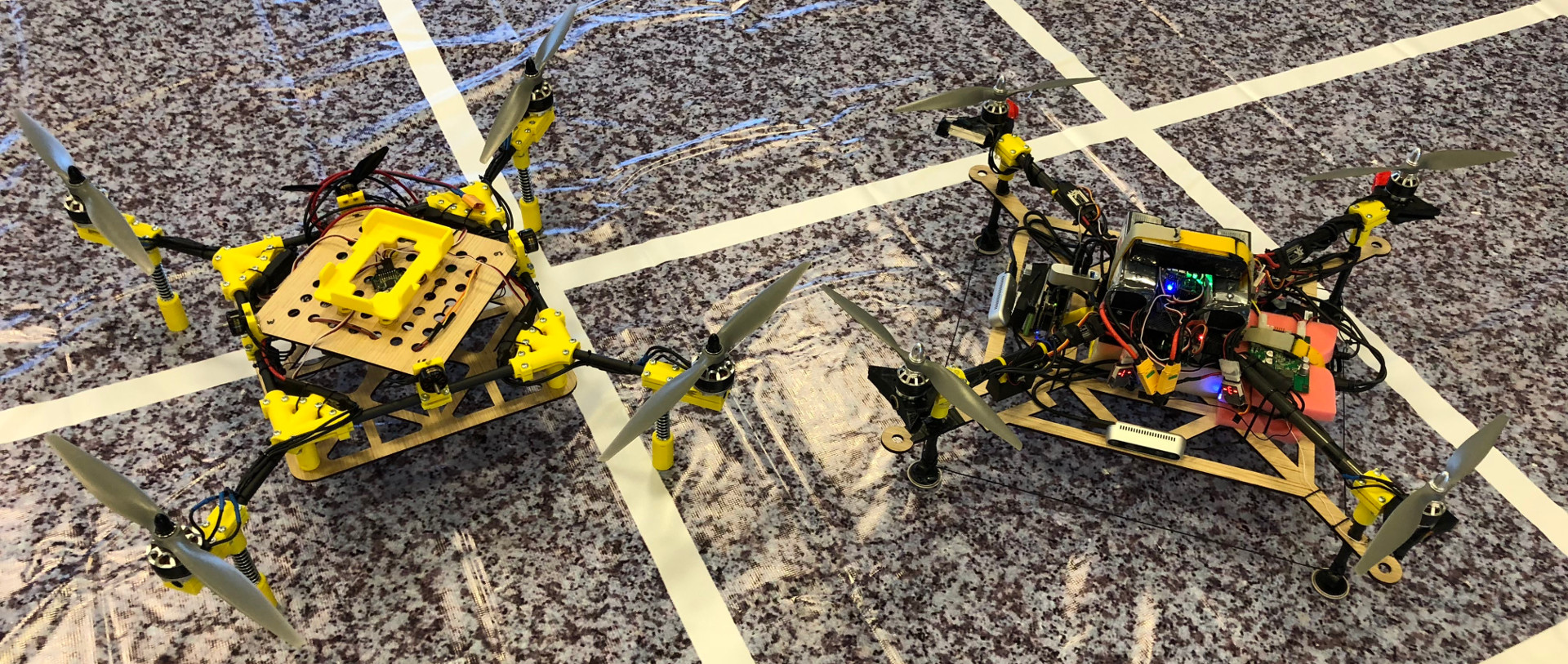
Left: UAV with 6 controllable degrees of freedom that was intended for the 2018 competition. Side propellers are not mounted.
Right: Actual drone used during the 2017 and 2018 competition (pictured for scale).

Significant effort was put into developing a new UAV for the 2018 competition year. The focus was a UAV with 6 controllable degrees of freedom. It would navigate without tilting by using 4 extra rotors mounted sideways. This would increase the positional maneuverability and allow for quicker ground target interaction.

A prototype was built and was demonstrated as part of Levi Burner, Long Vo, Liam Berti, and Ritesh Misra’s senior design project. Their demonstration video is embedded below. However, this prototype could not carry all of the electronics required for Mission 7. A model suited for Mission 7, pictured above, was built, however there was not time to migrate the computers and cameras to the new air frame.

Congratulations! You made it to the bottom. We hope you’ve had at least 1e-9 as much fun reading this as we’ve had over the last two years! Thanks for reading!